Remember that movie The Social Network from 2010? That was a solid one indeed. I liked the part where Andrew Garfield’s character said “I like standing next to you, Sean. It makes me look so tough.” That movie is 14 years old now. Let that sink in.

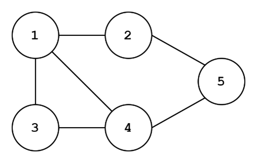
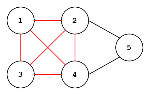
The reason I bring up The Social Network is that social networks are a great example of what we’re going to talk about today: GRAPHS. Graphs are data structures that made of nodes (or vertices) and edges (or links). I’m pretty sure using vertex or node doesn’t matter, and edge or link are also the same. So I will probably use both with no rhyme or reason throughout this piece. Here’s an example of a graph:

The nodes (represented as circles) are numbered from 1 to 5 and an edge is expressed as a line between two nodes. Edges generally denote some sort of relationship between two nodes. Get why a social network is an example of a graph? Think of people as nodes and if two people are followers or friends or whatever in a social media platform, they have an edge between each other. Graphs in computer science can be expressed a few different ways and not-so-surprisingly, different graphs represent different things. Here’s a mathematical definition of a graph:

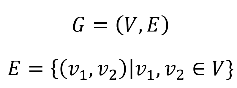
Very, very fancy. I will probably refer to nodes using their number and edges with the notation (node1, node2), where node1 and node2 are the nodes connected by the edge in question. I think this is pretty sufficient to get into the 10 miles wide part of this post. I’m going to run through a bunch of different types of graphs, key algorithms, and other graph stuff that comes to mind (not necessarily in that order).

Types

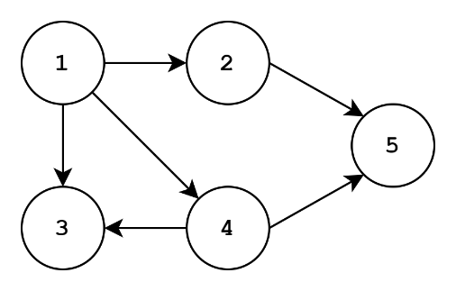
Undirected vs Directed

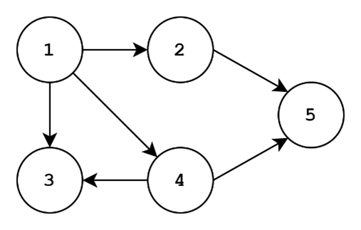
To the left, we have an undirected graph. To the right, we have a directed graph. Directionality is an attribute of the edges of a graph: each edge has a source and a destination node. The arrow of an edge points from source to destination. Undirected graphs have no directionality in their edges. The existence of an edge merely indicates the presence of some sort of relationship, with no assumption of directionality of that relationship. Our social network example of having friends may be represented by an undirected graph. However, a social network with followers could be modeled with a directed graph, since one person (source node) follows (directed edge) another person (destination node). Often times, folks will use the same notation for directed edges as I discussed before, with the caveat that the first node in (node1, node2) corresponds to the source node and the second will correspond to the destination in a directed graph. Thus, (node1, node2) is NOT equal to (node2, node1) in a directed graph, but these edges are equivalent in an undirected graph.

Unweighted vs Weighted

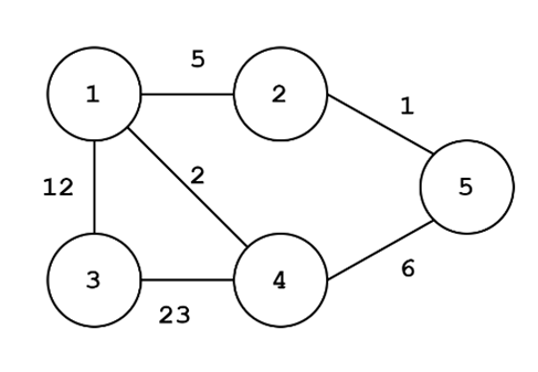
To the left, we have an unweighted graph. To the right, we have a weighted graph. Like directionality, weight is an attribute of edges. In an unweighted graph, each edge is assumed to have equal importance, or…you guessed it…weight. Weights can really shake some things up in terms of how algorithms traverse a graph, partition (split) the graph, or perform operations in general. For example, we might be interested in finding an unweighted graph split such that we maximize the number of edges that are removed, resulting in two partitions of the graph. When we transform the graph to a weighted graph, we might instead be interested in maximizing the weights that are cut. Take the unweighted graph on the left. We could cut the edges {(1,2), (1,4), (1,3), (2,5), (4,5)} which would be the maximum number of edges to cut to yield two separate partitions. For the weighted graph on the right, it might be a better idea to cut the edges {(3,4), (1,3), (4,5), (1,2)} since we are removing the weights 23,12,6,5 (summing to 46).

Acyclic vs Cyclic

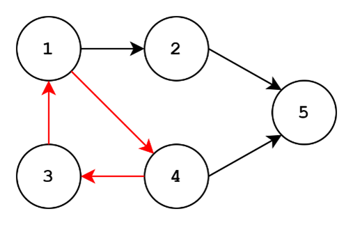
To the left, we have an acyclic graph. To the right, we have a cyclic graph. Cycles are trails or paths in the graph where the starting and ending nodes are equal. For the graph on the right, we can have the following path: 1->4->3->1. This is a cycle! For the graph on the left, the best we can do is 1->4->3, but we can’t go back to 1. In fact, we can’t end up back at any starting node for the graph on the left. Since there aren’t any cycles, the graph is acyclic.

Cycles can be a bit of a nuisance depending on the goal. If we are trying to traverse the graph, our algorithm better recognize that we’ve already visited a node or we might end up in an infinite loop!

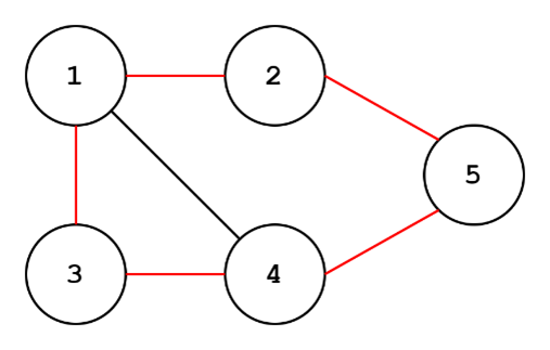
If you were wondering what a cycle looks like for a undirected graph, here it is. In this case, the cycle path can go either direction.

Bipartite Graphs

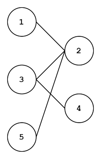
This graph looks a little funny. There are two disjoint sets of nodes ({1,3,5} and {2,4}). If you know some Latin or Greek root words, you might recognize that bipartite means something along the lines of “two parts”. A bipartite graph is a graph where nodes can be partitioned into two sets such that there are no edges between nodes in the same set. Think of modeling protein-gene interactions. One set (proteins) have edges (relate to) with another set (genes).

Trees

Trees kind of look like trees. Helpful, right? To be more accurate, trees are connected, acyclic, undirected graphs. “Connected” just means there’s at least one path from each node to every other node. With trees, adding the “acyclic” and “undirected” modifiers to “connected” implies that there is exactly ONE path from each node to every other node.

Trees are a whole beast with several variants, applications, and important algorithms. Unfortunately for you, you may have to do some further exploration. Here are some things that might help you get going:

1. In the CS data structure world, each node (except the topmost node (the root node)) has one parent.
2. Parents are closer to the root node compared to child nodes, or children.
3. When each node has at most two children, the tree is a binary tree.
4. All trees are bipartite!

File systems are a great example of a tree data structure, but not a binary tree!

Graph Things

I couldn’t decide whether to put this stuff under the Types category or not, so I went with or not. Here are some other graph things.

Cliques

Cliques are fully connected subgraphs (peep the set of nodes connected by red edges). Every node part of the clique is connected to every other node in the clique. These could have some implications depending on the application. Bipartite graphs have an analog called bicliques: https://en.wikipedia.org/wiki/Complete_bipartite_graph. Check out this page for more.

Algorithms

All this graph business is great and all, but who cares if you can’t do something with them?

Traversing graphs

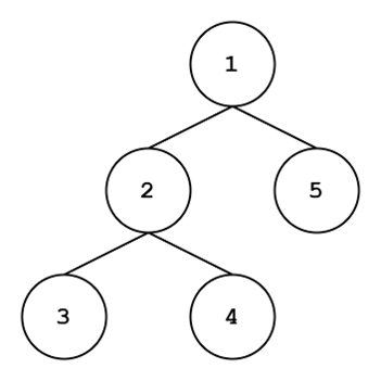
There are a few ways of traversing graphs, but we’re going to talk about the coolest ways: depth-first search (DFS) and breadth-first search (BFS). Check out the two trees just above. The tree on the top has a DFS traversal: when starting from the root node, we go as deep as we can and order our nodes in this fashion. Typically, if there are two children, we go down the left subtree first. The tree on the bottom is a BFS traversal: we visit all children of a level before going to the next level.

Though I’m showing trees here, we can extend this to any graph really. You probably should figure out a way to break ties for children of the same level though. Let’s do some traversing for this graph:

Let’s say we start at node 1. Our DFS traversal could be: 1, 2, 5, 4, 3. Generally, we don’t want to visit the same node twice, hence why we don’t have 1, 2, 5, 4, 5, 4, 3. Our BFS traversal could be: 1, 2, 4, 3, 5. Pretty interesting, right?

MaxCut

AHA! I already went over this one! Pulled a fast one there. Look at the Unweighted vs Weighted section, specifically where I talk about splitting the graph into two partitions. This is the MaxCut problem. Here’s the Wikipedia: https://en.wikipedia.org/wiki/Maximum_cut.

Max Clique

This one is fairly straightforward (https://en.wikipedia.org/wiki/Clique_problem). We want to figure out what the largest clique in the graph is, that is, the clique with the most nodes in a graph. There’s also the maximum biclique problem for bipartite graphs, with two versions: finding the biclique with the most edges and finding the biclique with the most nodes. These two versions are NOT the same.

Wrapping Up

Well, this was a lot. Graph theory is a lot. It’s still a hopping field, with applications ranging from social media to biology to deep learning. Hopefully this gave you a taste of the world within. Till next time.